
In today’s article we will focus on some common misperceptions of macroeconomics. Macroeconomics is the study of large-scale economic activity which includes the economy, the impact of the Federal Government’s policies and interactions between countries that affect employment, Gross Domestic Product (value of all goods and services produced during a given timeframe) and other factors such as interest rates and inflation.
Misconception 1: There is a common definition of what a recession is.
There is no common definition of recession across economists. The National Bureau of Economic Research (NBER) is a private, not for profit organization who has taken it upon themselves to be the arbiter for when recessions occur. In the past, it was generally understood that a recession occurred when there was reduction in GDP over two consecutive quarters. But this was not an official definition.
The NBER defines a recession as a “significant decline in economic activity that is spread across the economy, lasting more than a few months.” This is a subjective definition, and it can be used for both political as well as economic uses. In fact, according to the NBER, the last recession occurred during the COVID pandemic and lasted only two months, which was the shortest recession on record.
But even an objective measure such as saying a recession is a reduction in GDP over two consecutive quarters is not perfect, either, since it could be a very small reduction or it could be due to an increase in imports (imports are subtracted from GDP since the goods or services were produced elsewhere). So, we are stuck with the NBER’s squishy definition for now.
Misconception 2: Recessions in the US are unusual and therefore rare
The data on US economic activity is not perfect, and it is very difficult to analyze the further back in time we go. According to the NBER, since 1854 there have been 34 different periods in US history where their squishy definition of a recession applies. That would be a recession every 5 years on average.
If we go back in time, we find even more recessions. The first likely recession in the US occurred in 17851, a couple of years before the US Constitution was officially ratified and it lasted roughly four years. The next likely one occurred a year later in 1789 and again lasted for multiple years. The problem though, is that trying to get accurate data during those timeframes is difficult and subject to great error.
However, the point remains the same. Recessions in the US are not rare. Predicting when the next recession will occur is nearly impossible, but the next recession will happen.
Misconception 3: FDR’s New Deal dramatically improved GDP while significantly reducing unemployment
There is a common belief that during the 1930’s (also called the Great Depression) in the US that it took extreme Federal Government spending to increase GDP and reduce unemployment back down to acceptable levels. If you look up The Great Depression in the US, the first odd discrepancy you should find is the timing of it. Most sources say the Great Depression started in the fourth quarter of 1929 after the stock market crashed. But there are disagreements on whether it ended in 1939, 1940 or 1941. The second discrepancy you will notice is that depending upon the source you cite, unemployment and GDP numbers vary. However, they all show the same general trends so in this case, the specifics are important but do not change the result. For GDP (Gross Domestic Product) we will look both at Nominal GDP (GDP not adjusted for inflation) and Real GDP, that is GDP adjusted for inflation. Let’s look at the data.
Nominal GDP (In Billions) 2
| Year | Nominal GDP |
| 1929 | $103.6 |
| 1930 | $92.2 |
| 1931 | $77.4 |
| 1932 | $59.2 |
| 1933 | $57.2 |
| 1934 | $66.8 |
| 1935 | $74.3 |
| 1936 | $84.9 |
| 1937 | $93.0 |
| 1938 | $87.4 |
| 1939 | $93.5 |
| 1940 | $101.4 |
| 1941 | $112.5 |
| 1942 | $126.7 |
The first thing we notice is that Nominal GDP dropped significantly between 1929 and 1933 but did not even get back to its 1929 level until 1941, which is when the US was ramping up preparations for war.
Now let’s look at unemployment. The unemployment rate dramatically increased between 1929 and 1933 in response to the slowing economy. But the lowest the unemployment rate was on an annual average basis during the 1930s was 14.3% and did not get below 10% until 1941. In 1942, with the war in full force and with the military population growing to nearly 4 million, unemployment took a sharp drop.
Unemployment 3
| Year | Unemployment Rate |
| 1929 | 3.1% |
| 1930 | 8.7% |
| 1931 | 15.8% |
| 1932 | 23.5% |
| 1933 | 24.8% |
| 1934 | 21.6% |
| 1935 | 20.0% |
| 1936 | 16.8% |
| 1937 | 14.2% |
| 1938 | 18.9% |
| 1939 | 17.1% |
| 1940 | 14.5% |
| 1941 | 9.7% |
| 1942 | 4.7% |
But let’s also look at Real GDP. In economics, we prefer to look at data after it has been adjusted for inflation. But in the 1930s, there were six years when inflation was negative (or deflation). If we adjust the GDP using current data, we get the following Real GDP by year. This provides us with an even more interesting story. GDP, adjusted for inflation started at $1.2 Trillion in 1929 and after going down until 1933, only barely got above this level by the end of the decade. Deflation means that even though GDP went down and remained low, that buying power stayed roughly the same for the country.
Yes, millions and millions of people were unemployed, but those who were able to keep their job could buy more.
Real GDP (In Trillions) 4
| Year | Real GDP |
| 1929 | $1.2 |
| 1930 | $1.1 |
| 1931 | $1.0 |
| 1932 | $0.9 |
| 1933 | $0.9 |
| 1934 | $1.0 |
| 1935 | $1.1 |
| 1936 | $1.2 |
| 1937 | $1.3 |
| 1938 | $1.2 |
| 1939 | $1.3 |
| 1940 | $1.4 |
| 1941 | $1.7 |
| 1942 | $2.0 |
The story goes that during the Great Depression, FDR’s New Deal raised GDP and lowered unemployment. And indeed, unemployment did go down slightly from 24.9% to 14.6% by the end of the decade. But, who in today’s world would find 17%, or 19% or even 14% unemployment rates acceptable? No one.
So, what really happened? The Federal Government under FDR did increase government spending from $3 Billion to $9 billion. But this was still less than half of the Government spending level during much of the 1920s. The New Deal did provide Americans with optimism that the government was trying to do something about the Depression, but the New Deal had almost no impact on Real GDP and only minimal impacts on unemployment.
World War 2, and the need to take millions of working men and women for military needs out of the workforce reduced unemployment levels. In addition, ramping up the war machine and the infrastructure investments needed were the reasons that GDP rose and unemployment fell.

Misconception 4: There are good measures that are commonly used to analyze income inequality across countries

When you read articles about the problems with income inequality, there are usually a couple of measures that are used to discuss the phenomenon. These include measures that look at the percentage of consumption, income or wealth within a country by quintiles (20 percentage point categories). But the most used measure is the GINI index.
The GINI index measures income, wealth or consumption inequality within a country. It creates a number from 0 to 100% where 0 shows perfect equality and 100 shows perfect inequality with just a single individual owning everything.
Let’s take two hypothetical countries with two people each. In country A, both individuals make an income of $50,000 US. In this case, the GINI index would be 0 and there would be perfect equality of incomes within that country. In country B, one person makes $100,000 and the other makes $0 so the GINI index equals 100 with perfect income inequality. But some simple problems arise with such an approach.
Let’s look at a couple of modern GINI indexes. In 2022, Kyrgyzstan and Belgium both had a GINI index of 26.4. But the average monthly salary of people living in Kyrgyzstan is about $427 US per month (2025 data) while the average salary in Belgium is around $4,500 US. Likewise, the poverty rate in Kyrgyzstan was roughly 2.5 times higher than Belgium.
So, two countries with vastly different income and poverty levels can end up with the same GINI index. This leads to a fundamental problem with the GINI index: It tells you how incomes are distributed within a country but does not tell you about the relative differences across countries. One may think that is intrinsically important to have equality of incomes within a country, but does anyone really believe that the average Belgian is no better off than the average Kyrgyz?
The GINI index thus becomes a proxy for one’s views on inequality and not really an objective measure of inequality across countries. A good way to understand an individual’s preference here is to ask the following:
Which country with two people would be a better place to live, assuming equal purchasing power: Country A with both individuals making $40,000 in income or Country B with two individuals, one making $50,000 and one making $250,000?
To adjust for these problems, many variations in the standard GINI index have been proposed but to date none is widely used that fundamentally fixes the problem. The Lorenz curve is also used but it has the same flaw, since Kyrgyzstan and Belgium would show only slightly different metrics using that method.
Misconception 5: The Laffer Curve and Supply Side Economics have been disproven
There have been many claims, even from some high-level economists, that Supply Side Economics, and especially the Laffer Curve, have been shown not to work. Paul Krugman, a liberal economistAn economist is someone who More who wrote for years in the New York Times, is one such economistAn economist is someone who More. Most of his arguments are based upon broad based assumptions and a bias towards Keynesian economics.
So, what is Supply Side Economics at its simplest and does it work?
Very simply, instead of focusing on things that drive the demand for goods and services, Supply Side Economics focuses on the production side of the economy. It relies on policies that make it easier and less costly to produce goods and services, in an effort to reduce costs and expand output in the economy. At its basic, Supply Side Economics looks to reduce regulation, invest in human capital and business process improvements, tax reductions, improve incentives to work and provide inducements to invest in new capital to aid productivity.
Let’s go back to Macroeconomics 101 to see what the key differences are in the graphs between Keynesian (Demand side) and Supply Side Economics.
See graphs below
The first graph shows the classical Keynesian model for growing an economy during a recession or depression. The government spends more money or reduces taxes, causing aggregate demand to move from Aggregate Demand 1 to Aggregate Demand 2. This causes an increase in output AND an increase in prices.
The second graph shows how the economy grows under Supply Side Economics. By reducing regulation, reducing taxes, increasing capital infrastructure through lower costs, the supply curve moves from Aggregate Supply 1 to Aggregate Supply 2. This also causes output to increase but also causes prices to go down or remain the same, depending on the shape of the supply curve.
So, since Supply Side Economics gets you the same general output increases as Keynesian policies while not increasing prices, why wouldn’t it always be preferable? Well, sometimes it may take longer for the supply side effects to work their way through the system or maybe the government wants to target certain industries and not all for growth. For example, the US got out of the Great Depression through huge increases in government spending that focused on military spending for World War 2. In addition, Keynesians would say that during severe recessions or depression, prices are falling anyways (deflation) and therefore there is no need to worry about price increases.
On the other hand, if you use Keynesian policies when output is already high or when there is inflation in the system, it causes even more inflation to occur and can ultimately result in stagflation. In addition, once government officials start raising output through Keynesian policies, it is almost impossible for them to stop or reduce spending as there are now voting constituents who will demand that they keep spending even if it is harmful. When was the last time a government program was ended to slow down inflation?
So, both Keynesian and Supply side models have their advantages but also some disadvantages. There is not one economic model that works in every circumstance, yet you will hear proponents of every model (including Monetarists) who say their model is always correct.
Supply Side Economics is therefore a very important part of the toolkit of the Federal Government. Supply Side Economics has been accused of being “Trickle Down Economics”, meaning a top-down approach to managing the economy. But I believe this is totally false. Think of it this way. If you use Keynesian policies, the Federal Government decides where it wants to spend the money and who gets it. To me, the is the ultimate in Trickle Down Economics. With Supply Side policies, the cost of production inputs and regulations are usually (but not always) reduced across the board, helping most industries. Companies decide what to do with their investments after those policies are implemented. To me, Keynesian Economics is Trickle Down while Supply Side is Trickle Up.
Finally, we get to a discussion of the Laffer Curve, which has been around for nearly a hundred years but was more formally discussed by Art Laffer, an economistAn economist is someone who More who studied at Yale and Stanford. During the 1970s, while acting as a consultant with the Nixon administration, Laffer discussed a simple concept.
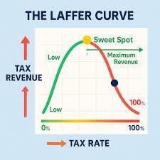
If the Federal Government imposes a federal income tax rate of zero, then it gets zero Federal revenues. On the other hand, if the Federal Government imposes a tax rate of 100%, then most people will stop working and revenues will decline or reach zero.
This implies there is a time when you raise tax rates that Federal revenues increase until there is a point when they start to go down. This seems intuitively obvious and indeed it is. The only real questions are what is the shape of the curve and what is the tax rate that maximizes revenue?
This implies there is a time when you raise tax rates that Federal revenues increase until there is a point when they start to go down. This seems intuitively obvious and indeed it is. The only real questions are what is the shape of the curve and what is the tax rate that maximizes revenue?
Laffer argues that this rate is much less than most economists think while others said that taxes can be raised almost to 100% before there is a problem. Laffer did not try to empirically prove his hypothesis since you would need multiple tax increases or decreases over a short period of time to prove it one way or another and Federal taxes fortunately do not change by large amounts in short periods of time.
Another concern is that you really cannot just look at Federal tax rates to determine the overall impact since all states have property taxes and most states have income and sales taxes which must be considered in any evaluation of the Laffer Curve. But having said that, the Laffer Curve has not been disproven and there is still a lot of work to understand the impacts of state and local taxes when discussing it.
Conclusion
In this blog, I discussed some basic misconceptions regarding macroeconomics including recessions, the New Deal, inequality measures and the Laffer Curve.
- Underwood, A (2022) stacker.com Every recession in U.S. history and how the country responded
- Calculated using multiple sources
- www.u-s-history.com
- Calculated using multiple sources and using 2025 dollars as a baseline